

3 - Sampling and Reconstruction
Understanding Sampling and Aliasing in Computer Vision (With Simple Examples)
Understanding Sampling and Aliasing in Computer Vision (With Simple Examples)
Meta Title
Sampling and Aliasing Explained (Computer Vision Basics with Python)
Meta Description
Learn sampling and aliasing in computer vision with simple explanations, real-life examples, and a beginner-friendly Python demo using scikit-learn.
What Is Sampling in Computer Vision?
Let’s start simple.
In computer vision, sampling is how we convert a continuous signal (like real-world light or sound) into something a computer can store and process.
Think about a real scene: light hits objects, reflects, and forms a smooth, continuous signal. But a camera doesn’t capture everything continuously—it records values at discrete points (pixels).
So instead of storing everything, we store snapshots at specific intervals.
👉 That process is called signal sampling.
Why Sampling Matters
Computers can’t store continuous data directly. They need numbers.
So we take a continuous signal and turn it into a set of values:
- A camera → samples light intensity across pixels
- A microphone → samples sound over time
- A sensor → samples measurements at intervals
But here’s the catch:
👉 Once you sample, you lose some information.
From Samples to Reconstruction
After sampling, we often want to reconstruct the original signal.
In simple terms:
We try to "connect the dots" between sampled values.
But we don’t actually know what happened between those points—we’re just estimating.
Simple Real-Life Example
Imagine this:
- You check the temperature only at 9 AM, 12 PM, and 3 PM
- You want to know how temperature changed between those times
You might draw a smooth curve between them—but that’s just a guess.
👉 That’s exactly what reconstruction does in computer vision and signal processing.
What Is Aliasing?
Now things get interesting.
Aliasing happens when we don’t sample enough.
If the sampling rate is too low, the reconstructed signal becomes incorrect or misleading.
Real-Life Example of Aliasing
Think about a spinning wheel in a movie:
- Sometimes it looks like it’s spinning backward
- Or slower than it actually is
That’s not real—it’s a sampling issue between frames.
👉 This is aliasing.
Understanding with a 1D Signal (Like Audio)
To make things easier, we often think in 1D signals (like sound over time).
One classic example is a chirp signal:
- Starts with low frequency
- Gradually increases to high frequency
If you played it, it would sound like a rising tone.
Why Chirp Signals Are Useful
A chirp contains many frequencies, so it helps us:
- Test how systems respond to different frequencies
- Observe where aliasing starts to happen
- Analyze signal behavior clearly
Python Example: Sampling and Aliasing (Beginner-Friendly)
Let’s look at a simple Python example using a generated signal.
We’ll:
- Create a continuous signal
- Sample it at different rates
- See what happens
import matplotlib.pyplot as plt
# Create a continuous signal (high resolution)
t = np.linspace(0, 1, 1000) # time axis
signal = np.sin(2 * np.pi * 10 * t) # 10 Hz sine wave
# Sample the signal at a lower rate
sample_rate = 20 # samples per second
t_sampled = np.linspace(0, 1, sample_rate)
signal_sampled = np.sin(2 * np.pi * 10 * t_sampled)
# Plot both signals
plt.figure()
# Original continuous signal
plt.plot(t, signal, label="Original Signal")
# Sampled points
plt.scatter(t_sampled, signal_sampled, label="Sampled Points")
plt.title("Sampling Example")
plt.xlabel("Time")
plt.ylabel("Amplitude")
plt.legend()
plt.show()
What’s Happening Here?
- The smooth curve = real (continuous) signal
- The dots = sampled values
- If we reduce
sample_rate, distortion appears
👉 That distortion is the beginning of aliasing.
Key Takeaways
- Sampling converts continuous signals into discrete values
- Reconstruction tries to estimate what’s between samples
- Aliasing happens when sampling is too low
- Higher frequency signals need higher sampling rates
Suggested Images (With Alt Text)
If you’re adding visuals to this blog, use:
- Smooth vs sampled signal graph
- Alt text: "Continuous signal compared with sampled discrete points"
- Aliasing example (distorted wave)
- Alt text: "Aliasing effect caused by low sampling rate"
- Chirp signal visualization
- Alt text: "Chirp signal with increasing frequency over time"
Internal Linking Suggestions
To improve SEO and user flow, link to related topics like:
- “Nyquist Theorem explained”
- “Image sampling in digital cameras”
- “Fourier Transform basics for computer vision”
- “How convolution works in image processing”
Where This Shows Up in Computer Vision
Sampling and aliasing appear in:
- Image resizing
- Texture rendering
- Camera sensor design
- Video frame capture
If you’ve ever seen jagged edges or flickering textures—that’s often aliasing.
Final Thoughts
Sampling sounds simple—just take values at intervals.
But the moment you try to reconstruct or analyze signals, things get tricky. You’re always balancing:
- Accuracy
- Storage
- Computation
And that’s where aliasing becomes important to understand.
So now we can start to talk about sampling and aliasing. So before we do that, we have to talk about the notion of sampling at all and the notion, and, and the idea of reconstruction. So here we have a the idea of some nice smooth scene illuminated by a light source and then we have an imaging system that captures the intensity at a bunch of discrete places.

And of course, what we'd like to do, is we'd like to take the captures from these discrete places, and be able to reconstruct this nice, smooth signal. That is to know what that signal is.
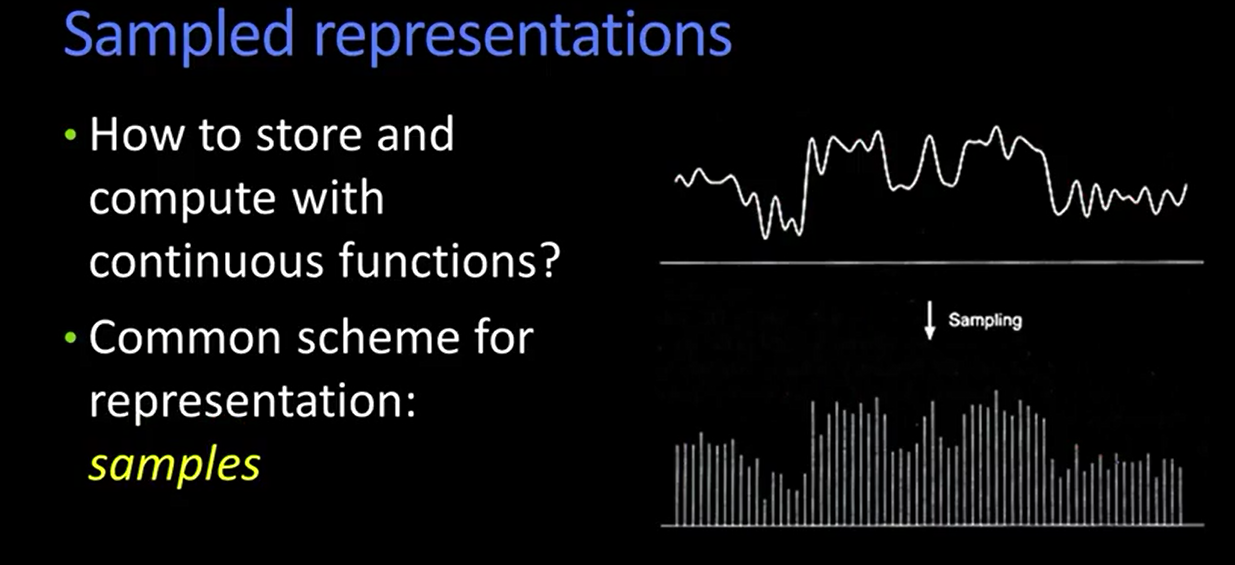
Let's talk a little bit about sampling. Sampling arises when we come up with this notion of, how do you store a continuous signal in a computer, right? So here we have a continuous signal, and this is in 1D, and we're going to do a lot of our stuff in 1D today because it's easier to draw. And so the obvious way of representing that, it's actually not the only way because you can imagine different clever basis kinds of things, but sort of a, a normal way of thinking about that is by samples. That is, you just take the samples at each different location and you write down what the value is.
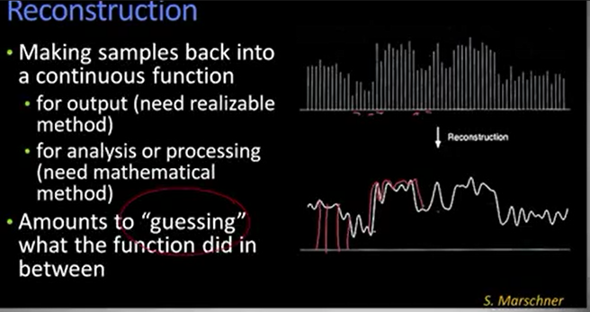
And once you have that set of samples later what you want to do is reconstruct what the original signal was, right? And why do you want to do this? Well, maybe you actually want to use the signal, you want to play it. If this is audio, you want to play it through a speaker. And I don't need samples, I need a continuous voltage. Or maybe I want to do some sort of analysis or a mathematical processing in terms of thinking about what this signal is. So essentially, what you have to do is you have to guess what's going on between each of the samples. That's all you can do. You have the samples at discrete places but you need to connect the dots if you will. You need to fill in what's going on. And a lot of what we're going to be talking about today has to do with what's actually going on, when you think about taking a set of samples and then trying to guess what's in between. So to illustrate most of these points we're going to use a 1B signal, so you think of this like audio, all right? So here's an interesting audio signal. You see this signal? This, so this is time, okay, it goes this way. And it starts off with a low frequency and it gets higher and higher and higher and higher, higher, higher and stops. All right, if you were to play that sound, you would hear what's called a chirp.
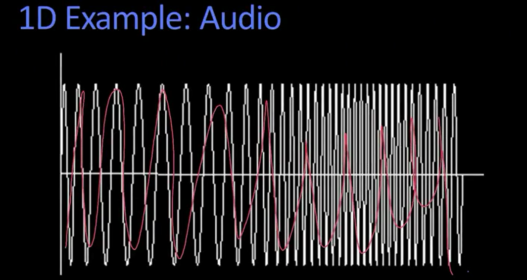
Okay, it's actually what it's called, it's called a chirp, it comes from radar, et cetera, whatever. It's something that has power in lots of different frequencies so when you send a chirp out, no matter what the frequency response of the thing you might be hitting is, you'll get something back. It also, it, it's also a nice way being able to localize it. There are lots of good reasons to use what's called a chirp. But here's a chirp that has higher and higher frequencies. But it's a good signal to think about looking at aliasing.