Classification Using PyCaret: A Beginner's Guide

Introduction 

Machine Learning (ML) is widely used for classification tasks, such as spam detection, sentiment analysis, and medical diagnosis. PyCaret, an open-source low-code ML library, simplifies classification by automating model selection, tuning, and evaluation. In this blog, we'll explore classification using PyCaret with a hands-on example.

Why Use PyCaret for Classification?

PyCaret provides a streamlined approach to ML workflows with features such as:

• Low-code implementation: Reduces the need for extensive coding.
• Automated preprocessing: Handles missing values, categorical encoding, and scaling automatically.
• Model comparison and selection: Evaluates multiple models and suggests the best one.
• Hyperparameter tuning: Optimizes model performance with minimal effort.
• Deployment-ready: Easily deploy models for real-world applications.

Import the necessary libraries

import numpy as np
import pandas as pd
import seaborn as sns
import matplotlib.pyplot as plt
from prettytable import PrettyTable
from sklearn.metrics import roc_curve, auc
from mlxtend.plotting import plot_confusion_matrix
from sklearn.model_selection import train_test_split
from sklearn.metrics import classification_report, confusion_matrix
from sklearn.tree import DecisionTreeClassifier
from sklearn.ensemble import RandomForestClassifier
from sklearn.svm import LinearSVC
from sklearn.linear_model import LogisticRegression
from sklearn.neighbors import KNeighborsClassifier
import warnings
warnings.filterwarnings("ignore")
#from pycaret.utils import enable_colab
#enable_colab()

Installing Pycaret

#capture #suppresses the displays # install the full version

!pip install pycaret[full]

Download Packages

 !pip install markupsafe==2.0.1

import pandas as pd
import numpy as np
import matplotlib.pyplot as plt
import seaborn as sns
import pycaret
import jinja2
#from pycaret.regression import*
from pycaret.classification import*
#pycaret.classification import *

Datasets

Let's use the famous Iris dataset, which is often used for classification tasks.

from pycaret.datasets import get_data
all_datasets = get_data()

In order to demonstrate the predict_model() function on unseen data, a sample of 1200 records has been withheld from the original dataset to be used for predictions. This should not be confused with a train/test split as this particular split is performed to simulate a real life scenario. Another way to think about this is that these 1200 records are not available at the time when the machine learning experiment was performed.

Setting up Environment in PyCaret

Common to all modules in PyCaret, the setup is the first and the only mandatory step in any machine learning experiment using PyCaret. This function takes care of all the data preparation required prior to training models. Besides performing some basic default processing tasks, PyCaret also offers a wide array of pre-processing features. To learn more about all the preprocessing functionalities in PyCaret, you can see this link. We use ‘pycaret.classification’ to set up with original dataset, target, and session_id. After we do it, we compare any models.

• Common to all modules in PyCaret, the setup is the first and the only mandatory step in any machine learning experiment using PyCaret.
• The setup() function initializes the environment in pycaret and creates the transformation pipeline to prepare the data for modeling and deployment.
• This function takes care of all the data preparation required before training models. Besides performing some basic default processing tasks, PyCaret also offers a wide array of pre-processing features
  
• setup() must be called before executing any other function in pycaret.
• It takes two mandatory parameters: a pandas dataframe and the name of the target column. All other parameters are optional and are used to customize the pre-processing pipeline.
• When setup() is executed, PyCaret's inference algorithm will automatically infer the data types for all features based on certain properties.
• The data type should be inferred correctly but this is not always the case. To account for this, PyCaret displays a table containing the features and their inferred data types after setup() is executed.
• If all of the data types are correctly identified enter can be pressed to continue or quit can be typed to end the expriment.
• Ensuring that the data types are correct is of fundamental importance in PyCaret as it automatically performs a few pre-processing tasks which are imperative to any machine learning experiment. These tasks are performed differently for each data type which means it is very important for them to be correctly configured.
• We use ‘pycaret.classification’ to set up with original dataset, target, and session_id. After we do it, we compare any models.

• I have passed log_experiment = True and experiment_name = 'diamond' , this will tell PyCaret to automatically log all the metrics, hyperparameters, and model artifacts behind the scene as you progress through the modeling phase. This is possible due to integration with
  
• Also, I have used transform_target = True inside the setup. Paret will transform the Price variable behind the scene using box-cox transformation. It affects the distribution of data in a similar way as log transformation (technically different).

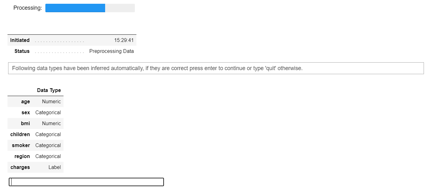
Once the setup has been successfully executed it prints the information grid which contains several important pieces of information. Most of the information is related to the pre-processing pipeline which is constructed when setup() is executed. The majority of these features are out of scope for the purposes of this tutorial however a few important things to note at this stage include:

• session_id: A pseduo-random number distributed as a seed in all functions for later reproducibility. If no session_id is passed, a random number is automatically generated that is distributed to all functions. In this experiment, the session_id is set as 123 for later reproducibility.

• Target Type : Binary or Multiclass. The Target type is automatically detected and shown. There is no difference in how the experiment is performed for Binary or Multiclass problems. All functionalities are identical.

• Label Encoded : When the Target variable is of type string (i.e. 'Yes' or 'No') instead of 1 or 0, it automatically encodes the label into 1 and 0 and displays the mapping (0 : No, 1 : Yes) for reference. In this experiment no label encoding is required since the target variable is of type numeric.

• Original Data : Displays the original shape of the dataset. In this experiment (22800, 24) means 22,800 samples and 24 features including the target column.

• Missing Values : When there are missing values in the original data this will show as True. For this experiment there are no missing values in the dataset.

• Numeric Features : The number of features inferred as numeric. In this dataset, 14 out of 24 features are inferred as numeric

• Categorical Features : The number of features inferred as categorical. In this dataset, 9 out of 24 features are inferred as categorical.

• Transformed Train Set : Displays the shape of the transformed training set. Notice that the original shape of (22800, 24) is transformed into (15959, 91) for the transformed train set and the number of features have increased to 91 from 24 due to categorical encoding

Notice how a few tasks that are imperative to perform modeling are automatically handled such as missing value imputation (in this case there are no missing values in the training data, but we still need imputers for unseen data), categorical encoding etc. Most of the parameters in setup() are optional and used for customizing the pre-processing pipeline. These parameters are out of scope for this tutorial but as you progress to the intermediate and expert levels, we will cover them in much greater detail.

2- Comparing All Models

• Now that data is ready for modeling, let’s start the training process by using compare_models function. It will train all the algorithms available in the model library and evaluates multiple performance metrics using k-fold cross-validation.

• Comparing all models to evaluate performance is the recommended starting point for modeling once the setup is completed (unless you exactly know what kind of model you need, which is often not the case). This function trains all models in the model library and scores them using stratified cross validation for metric evaluation. The output prints a score grid that shows average Accuracy, AUC, Recall, Precision, F1 and Kappa accross the folds (10 by default) of all the available models in the model library.

• This function trains all the available models in the model library using default hyperparameters and evaluates performance metrics using cross-validation.

• The number of folds can be defined using the fold parameter (default = 10 folds). The table is sorted (highest to lowest) by the metric of choice which can be defined using the sortparameter(in this case we have sorted it on RMSE) n_select parameter in the setup function controls the return of trained models. In this case, I am setting it to 15, meaning return the top 15 models as a list. pull function in the second line stores the output of compare_models as pd.DataFrame

• Two simple words of code (not even a line) have created over 15 models using 10 fold stratified cross validation and evaluated the 6 most commonly used classification metrics (Accuracy, AUC, Recall, Precision, F1, Kappa). 

• The score grid printed above highlights the highest performing metric for comparison purposes only. The grid by default is sorted using 'Accuracy' (highest to lowest) which can be changed by passing the sort parameter. 

• For example compare_models(sort = 'Recall') will sort the grid by Recall instead of Accuracy. If you want to change the fold parameter from the default value of 10 to a different value then you can use the fold parameter[5]

• If you want to change the fold parameter from the default value of 10 to a different value then you can use the fold parameter. For example compare_models(fold = 5) will compare all models on 5 fold cross validation. Reducing the number of folds will improve the training time.

best= compare_models(n_select = 2, sort= 'Accuracy')

3- Create a Model

• While compare_models() is a powerful function and often a starting point in any experiment, it does not return any trained models. PyCaret's recommended experiment workflow is to use compare_models() right after setup to evaluate top performing models and finalize a few candidates for continued experimentation.

• As such, the function that actually allows to you create a model is unimaginatively called create_model() [5]

• This function creates a model and scores it using stratified cross validation. Similar to compare_models(), the output prints a score grid that shows Accuracy, AUC, Recall, Precision, F1 and Kappa by fold

lda = create_model('lr')

 

• Notice that the mean score of all models matches with the score printed in compare_models(). This is because the metrics printed in the compare_models() score grid are the average scores across all CV folds. Similar to compare_models(), if you want to change the fold parameter from the default value of 10 to a different value then you can use the fold parameter. For Example: create_model('dt', fold = 5) will create a Decision Tree Classifier using 5 fold stratified CV. 

4- Tune a Model

we need to improve it with tune_model. It is a function that automatically tunes the model with hyperparameters.  When a model is created using the create_model() function it uses the default hyperparameters. In order to tune hyperparameters, the tune_model() function is used. This function automatically tunes the hyperparameters of a model on a pre-defined search space and scores it using stratified cross validation. The output prints a score grid that shows Accuracy, AUC, Recall, Precision, F1 and Kappa by fold.

Note: tune_model() does not take a trained model object as an input. It instead requires a model name to be passed as an abbreviated string similar to how it is passed in create_model(). All other functions in pycaret.classification require a trained model object as an argument.

tuned_lda= tune_model(lda, optimize='Accuracy', search_library='optuna')

tuned_lda= tune_model(lda, optimize='Accuracy', search_library='optuna')

tuned_dt = tune_model('dt')

Optimum Hyperparameters selected by using Optuna

5-Plot a Model

Before model finalization, the plot_model() function can be used to analyze the performance across different aspects such as AUC, confusion_matrix, decision boundary etc. This function takes a trained model object and returns a plot based on the test / hold-out set. There are 15 different plots available, please see the plot_model() docstring for the list of available plots. 

5.1 Analyze the best model

If we do not want to plot all these visualizations individually, then the PyCaret library has another amazing function — evaluate_model. In this function, you just need to pass the model object and PyCaret will create an interactive window for you to see and analyze the model in all the possible ways:

evaluate_model(lda)

5.2 Predict new Data

The predict_model() function is also used to predict on the unseen dataset. The only difference from section 11 above is that this time we will pass the data_unseen parameter. data_unseen is the variable created at the beginning of the tutorial and contains 5% (1200 samples) of the original dataset which was never exposed to PyCaret. (see section 5 for explanation) 

The Label and Score columns are added onto the data_unseen set. Label is the prediction and score is the probability of the prediction. Notice that predicted results are concatenated to the original dataset while all the transformations are automatically performed in the background.

5.3- Check the residuals of the trained model 

plot_model(best, plot = 'residuals_interactive')

5.4- Check feature importance

plot_model(lda, plot = 'feature')

5.4- Dashboard

5.5- Interpret the results

 we can interpret the model by SHAP values and correlation plot with just one line of code

5.6- AUC Plot

5.8- Precision-Recall Curve

5.9- Confusion Matrix

5.10- Cross-validation

Evaluate the model on the holdout set used for validation

6- Finalize and Save Pipeline

Let’s now finalize the best model i.e. train the best model on the entire dataset including the test set and then save the pipeline as a pickle file

Model finalization is the last step in the experiment. A normal machine learning workflow in PyCaret starts with setup(), followed by comparing all models using compare_models() and shortlisting a few candidate models (based on the metric of interest) to perform several modeling techniques such as hyperparameter tuning, ensembling, stacking etc. This workflow will eventually lead you to the best model for use in making predictions on new and unseen data. The finalize_model() function fits the model onto the complete dataset including the test/hold-out sample (30% in this case). The purpose of this function is to train the model on the complete dataset before it is deployed in production. 

final_best = finalize_model(lda) # save model to disk
save_model(final_best, 'diamond-pipeline')

save_model function will save the entire pipeline (including the model) as a pickle file on your local disk. By default, it will save the file in the same folder as your Notebook or script is in but you can pass the complete path as well if you would like:

save_model function will save the entire pipeline (including the model) as a pickle file on your local disk. By default, it will save the file in the same folder as your Notebook or script is in but you can pass the complete path as well if you would like:

We have now finished the experiment by finalizing the tuned_rf model which is now stored in final_rf variable. We have also used the model stored in final_rf to predict data_unseen. This brings us to the end of our experiment, but one question is still to be asked: What happens when you have more new data to predict? Do you have to go through the entire experiment again? The answer is no, PyCaret's inbuilt function save_model() allows you to save the model along with entire transformation pipeline for later use.

save_model(final_best, 'c:/users/moez/models/diamond-pipeline'

Caution: One final word of caution. Once the model is finalized using finalize_model(), the entire dataset including the test/hold-out set is used for training. As such, if the model is used for predictions on the hold-out set after finalize_model() is used, the information grid printed will be misleading as you are trying to predict on the same data that was used for modeling. In order to demonstrate this point only, we will use final_rf under predict_model() to compare the information grid with the one above in section 11. 

7- Loading the saved model

To load a saved model at a future date in the same or an alternative environment, we would use PyCaret's load_model() function and then easily apply the saved model on new unseen data for prediction.

References

1- PyCaret 101: An introduction for beginners

2-Auto_Model_Training_and_Evaluation_.ipynb

3-Build a machine learning model with PyCaret and corresponding user interface with Gradi

4-PyCaret in Machine Learning

5- Binary Classification Tutorial Level Beginner -  CLF101.ipynb