Introduction 

In the vast realm of computer vision, where algorithms and techniques constantly evolve, one fundamental operation stands out for its simplicity and effectiveness: scalar multiplication. This seemingly basic mathematical operation plays a pivotal role in manipulating and enhancing images, providing a versatile tool for a wide array of applications.

Sections

• Understanding Scalar Multiplication
• The Formula
• Enhancing Contrast
• Global and Local Adjustments
• Handling Saturation
• Implementation in Matlab
• Implementation in Python
• Conclusion

Section 1- Understanding Scalar Multiplication

Scalar multiplication involves multiplying each pixel in an image by a scalar value. This scalar can be any real number, and the operation is applied independently to each channel of a pixel (e.g., red, green, and blue in an RGB image). The beauty of scalar multiplication lies in its ability to scale the intensity values of an image without altering its structure.

Section 2- The Formula:

For a given pixel (R, G, B) and scalar value s, the scalar multiplication is performed as follows:

• New Red Value = R * s
• New Green Value = G * s
• New Blue Value = B * s

This operation can be extended to grayscale images as well, where each pixel's intensity is multiplied by the scalar.

Section 3- Enhancing Contrast

One of the most common applications of scalar multiplication in computer vision is contrast enhancement. By carefully selecting an appropriate scalar value, you can control the overall brightness and contrast of an image. Increasing the scalar will amplify the differences between pixel intensities, resulting in a more pronounced contrast.

Consider a photograph taken in low-light conditions. Applying scalar multiplication with a value greater than 1 will boost the pixel intensities, revealing details that might be lost in the original image. Conversely, using a scalar between 0 and 1 can tone down the intensity, reducing the overall contrast for a softer look.

Section 4- Global and Local Adjustments

Scalar multiplication can be applied globally to an entire image or locally to specific regions. Global adjustments affect the entire image uniformly, while local adjustments allow for fine-tuning in specific areas. This flexibility is particularly useful in scenarios where different parts of an image require distinct enhancements.

For instance, in medical imaging, where highlighting specific features is crucial, local adjustments with scalar multiplication can be employed to emphasize certain regions of interest while maintaining the overall context.

Section 5-Handling Saturation

Scalar multiplication also plays a role in adjusting image saturation. Saturation refers to the intensity of colors in an image. By applying scalar multiplication to the color channels, you can control the vibrancy of the colors. A scalar greater than 1 will intensify the colors, while a scalar between 0 and 1 will desaturate the image.

This property is valuable in fields like graphic design and digital art, where achieving a specific color palette is essential. It allows artists and designers to manipulate the saturation of an image without altering its other characteristics.

Section 6-Implementation in Matlab

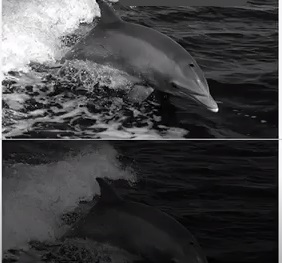
In the previous example, we saw how we can divide an image by a number. Dividing by 2 is the same as multiplying by 0.5. And the order of writing these two doesn't matter either. The constant 0.5 is known as a scalar. This potentially comes from the fact that it scales the image values.Let's see what the result looks like compared to the original image. Halve the intensity values, clearly darker.

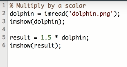
Note that we can potentially multiply by any number, even greater than 1. Multiplying the intensity values by 1.5 makes the image brighter.

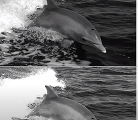
And we see the same washed out effect in certain areas. This is due to the image values above 255 getting truncated at that limit. In Octave, we can write a function to perform a common operation. Let's turn the scaling into a function. We write a function by typing in the word function, followed by a variable name for the return value. Then an equal sign, the name of the function, and parameters in parentheses. This is followed by the body of the function. In this case, we want the result to be the product of value and image. To ensure that we are performing element-wise multiplication, let's change the star to a dot star. This doesn't make any difference when one of the values is scalar, but when the two quantities being multiplied are vectors or matrices, then star and dot star produce different results. We end the function by typing end function. Let us load an image and try out this function. And there is the scaled image. 

Section 7- Implementation in Python 

Let's take a simple example using Python and the popular OpenCV library to perform scalar multiplication on an image:

import cv2 import numpy as np 
# Load the image image = cv2.imread("example.jpg") 
# Define a scalar value scalar = 1.5 
# Perform scalar multiplication
 result = np.clip(image * scalar, 0, 255).astype(np.uint8) 
# Display the original and modified images
 cv2.imshow("Original Image", image) 
cv2.imshow("Scaled Image", result) 
cv2.waitKey(0) 
cv2.destroyAllWindows()

Conclusion

Scalar multiplication may seem like a simple operation, but its impact on image processing and computer vision is profound. From enhancing contrast and adjusting saturation to performing local and global adjustments, scalar multiplication empowers developers, researchers, and artists with a powerful and intuitive tool. As the field of computer vision continues to advance, the role of fundamental operations like scalar multiplication remains pivotal in shaping the visual landscape of the digital world.

Reference