Machine Vision Applications

Here the interest is on procedures for the extraction of image information suitable for Computer processing ( To extract some Descriptions or some features which can be used for further processing by digital computer)

Typical Applications:

1- Industrial Machine vision for product assembly and inspection 

such a kind of processing can be applied in industrial machine vision for the product, assembly, and inspection.

2. Automated target detection and tracking

3. Fingerprint recognition

4. Machine Processing of aerial and satellite images, for weather predictions, crop assessment, and man other  applications

1- Industrial Machine vision for product assembly and inspection 

  Inspection 

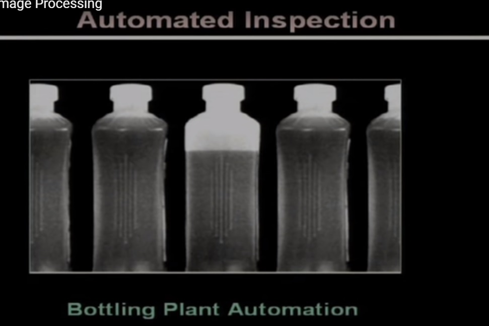
This shows an application of automation of a bottling plan; here what the plant does is, fills up some liquid. some chemical into a bottle and after it is filled up, the bottles are carried away by the conveyor belts and after these are packed and finally sent to the customers. So here checking the quality of the product is very important and in this particular application, the quality of the product indicates that whether the bottles are filled properly or some bottles are coming out empty or partially filled. So naturally, the application will be that if we can find out that some bottles are partially filled or some bottles are empty then naturally we do not want those bottles to be delivered to the customer because if the customer gets such bottles then the goodwill of the company would be lost  So the detection of the empty bottles or partially filled bottles is very, very important, and here image processing techniques can be used to automate this particular process so here you find that we have shown an image the snapshot of this bottling process where you find that there are some bottles which are completely filled up and one bottle in the middle which is partially filled. So naturally, we want to detect this particular bottle and remove it from the production line so that finally when the bottles go to the customer no empty bootle or no partially filled bottle are given to the customer.

Boundary information

There is another application in machine vision, for machine vision purposes. Now before I go to that application, I have shown an image to highlight the importance of boundary information in image processing. So here you find we have shown the boundary image of the animal there is no other information available in this image except the boundary counters. And you find that if I asked you can you identify this particular animal and I am sure

That all of you will identify this to be a giraffe, So you find that even though we do not have any other information except the boundary or the border of the giraffe, but still we have been able to identify this particular animal. So in many cases or in most of the cases the boundaries contains most of the information of the objects present in the scene and using this boundary information so we can develop the various application of image processing techniques.

Here is an application :

so this is again an automated inspection process and here the objects that we are interested to inspect are some refractory bricks. So here we find that we have shown 4 different images. The first one is the original image which is of the refractory brick which is captured by the camera. The second one is what we call is a threshold image or a segmented image we come to details of this later where we have been able to identify that what are the regions which actually belong to this projects and what are the regions which belong to the boundary. Naturally, when we are interested in inspecting this particular object we will not interested in the background region.

So this background and object separation process is very, very important in all these kind of applications. The third image, that is the left one on the bottom is a field image. You find the second image; it is not very smooth. There are a number of black patches over the white region. So the second one has filled up all those black patches and it shows that what is the profile of the object, the 2D projection of the object that we can get. And the fourth image, you will find that it shows that what is the boundary of this object. And using this boundary information we can inspect various properties of this particular object. For example, in this particular application, there can be

Two different types of defects.

One kind of defect is the structural defect. When we say the structural defect, by structure what I mean is, what is the dimension of every side of the object, what is the angle at every corner of the object. These are the structural information of that particular object.

And the other kind of inspection that we are interested to do is what is the surface characteristics of this particular object, whether the surface is uniform or the surface is non-uniform. So let us see that how these inspections can be made.

So here you find that the first image, what we have done is we have processed the boundary image in such a way that since there are 4 different boundary regions, we have fitted 4 different straight lines and these 4 different straight lines; that tells you that what should be the ideal boundary of the object. And once we get these 4 different straight lines, using these 4 different straight lines we can find out what are the points of intersections of these 4 different straight lines. And using these point of intersections we know that in the ideal situation, those points of intersections are actually the locations of the corners of the object. So you find that in the first image, there are 4 white dots which indicates the corners of the object. And once we get these informations, the corners of the object, the boundary line of the object, we can find out what is the dimension of or the length of each and every side of the object. We can also find out, what is the corner subtended, what is the angle subtended at every corner of the object and from this, if I compare the information that we have obtained through image processing with the information which is already stored in the database for this particular object, we can find out whether the dimensions that we have got is within the tolerable limit or not. So if it is within the tolerable limit then we can accept the object. If it is not within the tolerable limit then we will not accept the object.

Now if you look at the original image once more you will find that there are two different corners, the right, the corner on the right-hand side, and the corner on the left-hand side. These corners are broken. Not only that, on the left-hand side, if you look at the middle, you can identify that there is a certain crack. So these are also the defects of this particular object and through this image processing technique, we are interested to identify these defects. Now let us see that how these defects are being identified. So here again in the first image, once we have got the ideal boundary and the ideal corners of the object, we can fill up the region bounded by these 4 different edges to get an ideal projection of the object. So the second image in this particular slide shows you that what is the ideal projection; the third image that shows you that what is the actual projection that has been obtained after image processing techniques. Now if this ideal projection, if we take the difference of this ideal projection and the actual projection then we can identify these defects. So you find that in the fourth image the two different corner bricks have been represented by white patches, also on the left-hand side in the middle, you have, you can see that the crack is also identified. So these image processing techniques can be used for inspection of industrial objects like this. And as we mentioned.

9,50

The other application or the other kind of inspection that we are interested in is the surface
characteristics, whether the surface is uniform, or the surface is non-uniform.

 Surface characteristics

So when we want to find out or study the surface characteristics, the type of processing technique that will be used is called texture processing. And this one shows that  for the surface of the object it is not really uniform, rather it contains 2 different textures and in the right image those 2 textures are indicated by 2 different gray shades.

It shows the application of image processing techniques for automated inspection in other applications. For example, the inspection of Integrated Circuits during the manufacturing phase. Here you find that in the first image, there is a broken bond where as in the second image some bond is missing which should have been there. So naturally these are the defects which are to be identified because otherwise, if this IC is made, then the IC will not function properly. So those are the applications which are used for machine-vision applications, for automating some operations and in most of cases, it is used for automating the inspection process or automating the assembly process.

Now we have another kind of application by processing the sequence of images that are known as a video sequence.

 Video sequence:

The video sequence is nothing but the different image frames which are displayed one after another. So naturally when the image frames are displayed one after another then if there is any movement in the image that movement is clearly detected. So the major emphasis in image processing, image sequence processing is to detect the moving parts. This has various applications. For example, detection and tracking of moving targets major applications are in security surveillance. to find the trajectory of a moving target. Also monitoring the movement of organ boundaries in medical applications is very, very important and all these operations can be done by processing video sequences. So let us take one such example.

 

Here you find that in the first image some person is moving against a green background. So
let us see this. So here we find that a person is moving against a background. So through image processing techniques we can identify this movement. So, in the second processed sequence you find that the person is moving which is clearly shown against a black background. That means we have been able to separate the background from the moving object.  Now this particular application which has been shown, here the image was taken or the video sequence was taken on broad daylight. But in many applications, for example, particularly for security applications, the images are to be taken  during the night also, when there is no sunlight. Then what kind of image processing techniques can be used for such surveillance applications? So here you find that we have shown an image

which is or a sequence  which is taken during the night and the kind of imaging that you have to take is not the ordinary optical imaging but here we have to go for infrared imaging or thermal imaging. So this particular sequence is a thermal sequence. So again here you find that a person is moving against a still background. So if you just concentrate in this region you find that the person is moving. And again through image processing techniques, we have identified just this moving person against the still background So here you find that the person is moving and the background is completely black. So these kinds of image processing  techniques can also be used for video sequence processing. Now let us take, look at another application of this image processing technique.

 

Now let us take, look at another application of this image processing technique. 

But even after changed shape, we have been able to track this particular object. But when the
object cannot be matched any further, the shape has changed so much 

that the object cannot be matched any further, it indicates poor detection. So what is the
application of this kind of image processing techniques? Here the application is, if I track this
moving object using a single camera, then with the help of a single camera, I can find out
what is the azimuth and elevation of that particular object with respect to certain reference
coordinate system. If I track the object with 2 different cameras and find out the azimuth and
elevation with the help of 2 different cameras then I can identify that what is the x, y, z
coordinate of that object with respect to that 3D coordinate system. And by locating those
locations in different frames, I can find out that over the time which path the object is
following and I can determine that what is the trajectory that the moving object follows. So
these are the different applications of video sequence processing.

Azimuth and Elevation are measures used to identify the position of a satellite flying overhead. Azimuth tells you what direction to face and Elevation tells you how high up in the sky to look. Both are measured in degrees. Azimuth varies from 0° to 360°.

So we have mentioned that we have a third application which is compression

and in compression what we want is, we want to process the image to reduce the space
required to store that image or if want to transmit the image we should be able to transmit the
image over a low bandwidth channel. Now let us look at this image and let us look at the
region, the blue circular region. You will find that in this particular region, the intensity of the
image is more or less uniform. That is, if I know that the intensity of the image at a particular
point, I can predict what is the intensity of its neighboring point. So if that prediction is
possible then it can be argued that why do have to store all those image points? Rather I store
one point and the way it can be predicted, its neighborhood can be predicted, we just mention
that prediction mechanism. Then the same information can be stored in a much lower space.
You will find this second region. Here again in most of the regions you find that intensity is
more or less uniform except certain regions like eye, like the hat boundary, like the hair and
things like that. So these are the kind of things which are known as redundancy.

So whenever we talk about an image, the image usually shows 3 kinds of redundancies. The
first kind of redundancy is called a pixel redundancy which is just shown here.

The second kind of redundancy is called a coding redundancy and the third kind of
redundancy is called a psychovisual redundancy. So these are 

the 3 kind of redundancies which are present in an image So whenever we talk about an
image

the image contains two types of entities, the first one is the information content of the image
and the second one is the redundancy and these are the three different kinds of redundancies.
So what is done for image compression purposes, you process the image and try to remove
the redundancy present in the image, retain only the information present in the image. So if

we retain only the information, then obviously the same information can be stored using a
much lower space. The applications of this are reduced storage as I have already mentioned

if I want to store this image on a hard disk, or if I want to store a video sequence on a hard
disk, 

then the same image or the same digital video can be stored in a much lower space.

The second application is reduction in bandwidth. 

That is if I want to transmit this image over a communication channel or if I want to transmit
the video 

over a communication channel then the same image or the same video will take much lower
bandwidth of the communication channel. Now given all these applications, this again shows
that 

what do we get after completion? So here we find that we have the first image which is the
original image, the second one shows the same image but here it is compressed 55 times. So
you find, if I compare the first image and second image, I find the visual quality of the two
images are almost same, at least visually we cannot make much of difference. Whereas if you
look at the third image which is compressed 156 times, now if you compare third image with
the original image you will find that in the third image there are a number of blocked regions
or blocking, these are called blocking artifacts which are clearly visible when you compare it
with the original image. The reason is, as we said that the image contains information as well
as redundancy. So if I remove the redundancy, maintain only the information then the
reconstructed image does not look much different from the original image. But there is
another kind of compression techniques which are called lossy compression. 

In case of lossy compression, what we remove is not only the redundancy but we also remove
some of the informations, so that after removing those informations the quality of the
reconstructed image is still acceptable. Now in such cases, because you are removing some of
the information which is present in the image so naturally the quality of the reconstructed
image will not be as the original image. So naturally there will be some loss or some
distortion and this is taken care by what is called rate distortion theorem.

Now if I just compare the space requirement of these 3 images, if the original image is of
size, say 256 by 256 bytes Ok that is 64 kilo bytes, the second image which is compressed 55 

times, the second image will take slightly above something around say 10 kilo bytes, Ok. So
you find that the difference. The original image takes 64 kilo bytes but the second one takes
something around 10 kilo bytes where as the third one will take something around 500 bytes
or even less than 500 bytes. So you will find that how much reduction in the space
requirement we can achieve by using these image compression techniques.

So given these various applications

now let us look at some history of image processing. Though the application of image
processing has become

very, very popular for last 1 or 2 decades but the concept of image processing is not that
young. In fact, as early in 1920s image processing techniques were being used. And during
those days, the image processing techniques or the digital images were used to transmit the
newspapers pictures between London and New York. And these digital pictures are carried
by submarine cables; the system which was known as Bartlane Systems. Now when you
transmit these digital images via a submarine cable then obviously on the transmitting side I
have to have a facility for digitization of the image, similarly on the receiving side, I have to
have a facility for reproduction of the image. So in those days, on the receiving side

the pictures are being reproduced by the telegraphic printers and here, find a particular
picture which was reproduced by a telegraphic printer.

Now next in 1921, there was improvement in the printing procedure. In the earlier days,
images were reproduced by telegraphic printers. In 1921 what was introduced was the
photographic process of picture reproduction. And in this case, on the receiver, instead of
using the telegraphic printer, the digital images or the codes of the digital images were
perforated on a tape and photographic printing was carried on using those tapes. So here you
find that there are 2 images, the second image is obviously the image that we have shown in
the earlier slide. The first image is the image which has been produced using this
photographic printing process. So here you find that the improvement both in terms of tonal
quality as well as in terms of resolution is quite evident. So if you have compared the first
image and the second image, the first image appears much better than the second image.

Now the Bartlane System that I said which was being used during 1920s that was capable of
coding 5 distinct brightness levels. This was increased to 15 levels by 1929, so here you find
an image with 15 different intensity levels and here the quality of this image is better than the
quality of the image which was produced by the Bartlane system. Now since 1929 

for next 35 years, the researchers have paid their attention to improve the image quality or to
improve the reproduction quality. 

And in 1964, these image processing techniques were being used by, in, at Jet propulsion
laboratory to improve the pictures of moon which have been transmitted by Ranger 7. And
we can say this is the time from where 

the image processing techniques or the digital image processing techniques has got a boost.
And this is considered to be the basis of modern image processing techniques. Now given the
applications as well as

and the history of image processing techniques, now let us see that how an image is to be
represented in a digital computer. This representation is very, very important because unless
we are able to represent the image in a digital computer, obviously we cannot process the
image. So here you find that we have shown an image and at a particular point x, y in the
image conventionally the x coordinate is taken vertically downwards and the y axis is taken
horizontally towards right. And if I look at this image this image is nothing but a two
dimensional intensity function Ok which is represented by f(x, y). Now if at any particular
point x, y we find out the intensity value which is represented by f(x, y), this f(x, y) is nothing
but a product of two terms. So here you find that this f(x, y) is represented by the product of
two terms one term is r(x, y) and other term is i(x, y). This r(x, y) is the reflectivity of the
surface of the corresponding image point Ok. After all, how do we get an image or how do
we, how can we see an object? You find that there must be some light source. If I take an
image in the daylight this light source is usually the sun, so the light from the light source
falls on the object surface. It gets reflected, reaches our eye and then only we can see that
particular object. So here you will find that this r(x, y) that represents that reflectivity of the
point on the object surface which is used from where the light gets reflected and falls on the
image intent. And this i(x, y), it represents the intensity of the incident light. So if I take the
product of the reflectivity and the intensity, these two terms are responsible for giving an
intensity at a particular point in the image. Now if we look at this, you find if this is an analog
image then how many points we can have on this image? Obviously there are, there is
information at every possible point both in the x direction and the y direction. That means
there are infinite number of points in this particular image. And at every point the intensity
value is also continuous between some minimum and some maximum and theoretically the
minimum value can be 0 and the maximum value can be infinite. So can we represent or can
we store such an image in a digital computer where I have infinite number of points and I
have infinite possible intensity values? Obviously not! So what we have to do is, we have to
go for some processing of this image

and what we do is, instead of storing all the intensity values of all possible points in the
image we try to take samples of the image on a regular grid. So here the grid is superimposed
on this particular image and what we do is we take samples, image samples at various grid
points, Ok. So the first level that we need for representation of an image in a digital computer
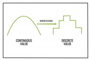
is spatial discretization by grids. And once we get these sample values, at every point the
value of that particular sample is again continuous. So it can assume any of the infinite
possible values, which again cannot be represented in a digital computer. So after sampling
the second operation that we have to do is discretization of the intensity values of different
samples, the process which is called quantization.

So effectively what we need is an image is to be represented by a matrix like this, Ok. So this
is a matrix of finite dimension. It has m number of rows and n number of columns. Typically
for image processing applications, the image size which is used is either 256 x 256 elements,
512 x 512 elements, 1 K x 1 K elements and so on. Each of these elements in this matrix
representation is called a pixel or a pel. Now, quantization of these matrix elements, now you
find that each of these locations represents a particular grid location where I have to, I have
stored a particular sample value. Each of these sample values are quantized and typically for
image processing applications, the quantization is done using 8 bits for black and white
image and using 24 bits for color image. Because in case of color, there are 3 color planes
red, green and blue. For each of the planes, if I use 8 bits for quantization, then it gives us 24
bits which is used for representation of digital color image.

So here you find that we just show an example that given this image if I take a small
rectangular area somewhere here, then intensity values of that rectangular area is given by a
matrix like this.

Now let us see what are the steps in digital image processing techniques. Obviously the first
step is image acquisition. The next step after acquisition is we have to do some kind of
processing which are known as preprocessing which takes care of removing the noise or
enhancement of the contrast and so on. The third operation is segmentation that is
partitioning an input image into constituent parts of objects. This segmentation is also
responsible for extracting the object points from the boundary points.

After segmentation, the next step is to extract some description of image objects which are
suitable for further computer processing. So these steps

are mainly used for machine vision applications Then we have to go for recognition. So once
we get description of the objects, from those descriptions we have to interpret or recognize
what the object is. And the last step is

the knowledge base, what the knowledge base helps for efficient processing as well as inter-
module cooperation of all the previous processing steps.

So here we have shown all those different steps with the help of a diagram where the first
step is image acquisition, the second step is preprocessing, then go for segmentation, then go
for representation and description and finally go for recognition and interpretation and you
get the image understanding result. And at the core of the system, we have shown a
knowledge base and here you find that the knowledge base has a link with all these different
modules, so the different modules can take help of the knowledge base for efficient
processing as well as for communicating or exchanging the information from one module to
another module. So these are the different steps 

which are involved in digital image processing techniques and in our subsequent lectures we
will elaborate on these different processing steps one after another. Thank you.