Reading
1. What is a Neural Network?
a neural network is made up of neurons connected to each other; at the same time, each connection of our neural network is associated with a weight that dictates the importance of this relationship in the neuron when multiplied by the input value. Each neuron has an activation function that defines the output of the neuron. The activation function is used to introduce non-linearity in the modeling capabilities of the network. We have several options for activation functions [1]. It resembles the brain in two respect. Knowledge is acquired by the network through a learning process (Called training ). Interneuron connection strengths are used to store knowledge. Knowledge is implicit and distributed. A neural network is a network of neurons, or in a modern sense, an artificial neural network, composed of artificial neurons. It mimics the brain's neurons using nodes, connections, and weights to find an output relative to a specific input. A neural network is based on a collection of connected units or nodes called artificial neurons, which loosely model the neurons in a biological brain. Each connection, like the synapses in a biological brain, can transmit a signal to other neurons. An artificial neuron that receives a signal then processes it, can send another signal to the neurons connected to it. Such a system " Learn " to perform tasks by considering example, generally without being programmed with task-specific rules.
2 Transfer Function or Activation Function
Remember that we use the activation functions to propagate the output of a neuron forward. This output is received by the neurons of the next layer to which this neuron is connected (up to the output layer included). As we have said, the activation function serves to introduce non-linearity in the modeling capabilities of the network. Below we will list the most used nowadays; all of them can be used in a layer of Keras
2.1. Sigmoid Function :
it converts independent variables of almost infinite range into simple probabilities between 0 and 1. Most of its output will be very close to the extremes of 0 or 1 [5]. The sigmoid function is a logistic function, which means that, whatever you input, you get an output ranging between 0 and 1. That is every neuron, node or activation that you input, will be scaled to a value between 0 and 1[6]. The sigmoid is often called a nonlinearity, simply because we cannot describe it in linear terms. Many activation functions are nonlinear, or a combination of linear and nonlinear – and it is possible for some of them to be linear, although that is unusual[6]. If you need binary classification then the sigmoid function is the best choice just in the output layer and never used in other hidden layers. In this function, the center of data is always close to 0.5
2.2 Tanh Function?
t Unlike the sigmoid function, the normalized range of
tanh is between -1 and 1, which is the input that goes well with some neural
networks. The advantage of tanh is that negative numbers can be dealt with more
easily [5]. it also works better than the sigmoid function because in this
center of data is closed to zero means and it makes learning easy for the next
layers. it is also a good choice in hidden layers not in output layers.
2.3 Softmax
instead of classifying in binary it can contain multiple decision limits. As we have seen, the softmax activation function will often be found in the output layer of a neural network and return the probability distribution over mutually exclusive output classes [5]
2.4 ReLU
The activation function rectified linear unit (ReLU) is a very interesting transformation that activates a single node if the input is above a certain threshold. The default and more usual behavior is that, as long as the input has a value below zero, the output will be zero but, when the input rises above, the output is a linear relationship with the input variable of the form f(x)=x. The ReLU activation function has proven to work in many different situations and is currently widely used [5]. The derivative is 1 when z is positive and the slop is zero when z is negative. If you doing binary classification then the sigmoid activation function is a good choice for the output layer and for all other units, RELU is a good choice. The downside is that derivative is zero when z equal to -1, therefore, we used another leaky RELU. Learn much faster because their slop is not going to zero like other functions.
2.5 Downside of sigmoid and Tangent
if Z is very large or small then gradient or derivative or slop of this function because small and due to this Gradient become slow
3. A neuron
It is a bloc of mathematical operations linking between entities [2]
4. Loss or Cost Function
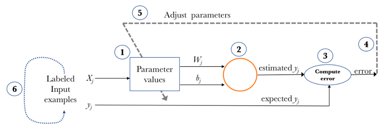
loss function to estimate the loss (or error) and to compare and measure how good/bad our prediction result was in relation to the correct result. Ideally, we want our cost to be zero, that is, without divergence between estimated and expected value. Therefore, as the model is being trained, the weights of the interconnections of the neurons will gradually be adjusted until good predictions are obtained [1]
5. ANN Training
5.1 Random initialization [8]
For logistic regression (LR) weight initialization with zero is ok; but; For the neural network (NN); it is important that weights are initialized randomly. If you apply zero in ANN and then Grediecent cannot work. In ANN; zero initialization for b is ok, but for W; it will create a problem. In ANN; If we initialized W and b with zero; then for all examples the activation of the hidden layer is equal or Symantec( a1^[1]=a2^[1]). for al example dz1^[1]=dz2[1]. After every single iteration of training of two hidden units still computing exactly the same function. After every iteration, the first row of the new W metric will equal to the second row. Every hidden layer in the first hidden layer gives the same effect on the output layer. How long you run gradient all hidden units produced exactly the same results. when different hidden units compute the same thing; This is also called a symmetry-breaking problem.

We iniliazation w with very small random value; if the weight is too large, then Z be very big or either very small or very big and finally, the activation function (sigmoid or tanh) will flat. Then gradient or slop will be zero or small. It meaning that learning will be slow. if shallow network the constant 0.01 is ok and for the deep network, we used different constant

5.2 Forward propagation
Forward propagation occurs when the network is exposed to the training data and these cross the entire neural network for their predictions (labels) to be calculated. That is, passing the input data through the network in such a way that all the neurons apply their transformation to the information they receive from the neurons of the previous layer and sending it to the neurons of the next layer. When the data has crossed all the layers, and all its neurons have made their calculations, the final layer will be reached with a result of label prediction for those input examples [1]
5.3 Backpropagation
Once the loss has been calculated, this information is propagated backward. Hence, its name: backpropagation. Starting from the output layer, that loss information propagates to all the neurons in the hidden layer that contribute directly to the output. However, the neurons of the hidden layer only receive a fraction of the total signal of the loss, based on the relative contribution that each neuron has contributed to the original output. This process is repeated, layer by layer, until all the neurons in the network have received a loss signal that describes their relative contribution to the total loss [1] . Now that we have spread this information back, we can adjust the weights of connections between neurons. What we are doing is making the loss as close as possible to zero the next time we go back to using the network for a prediction. For this, we will use a technique called gradient descent. This technique changes the weights in small increments with the help of the calculation of the derivative (or gradient) of the loss function, which allows us to see in which direction “to descend” towards the global minimum; this is done in general in batches of data in the successive iterations (epochs) of all the dataset that we pass to the network in each iteration [1]
6. Learning Steps of ANN [1]
- Start with values (often random) for the network parameters (wij weights and bj biases).
- Take a set of examples of input data and pass them through the network to obtain their prediction.
- Compare these predictions obtained with the values of expected labels and calculate the loss with them.
- Perform the backpropagation in order to propagate this loss to each and every one of the parameters that make up the model of the neural network.
- Use this propagated information to update the parameters of the neural network with the gradient descent in a way that the total loss is reduced and a better model is obtained.
- Continue iterating in the previous steps until we consider that we have a good model.