• Frequency in Images (Outside Knowledge): In audio, high frequency means a high-pitched sound. In an image, "high frequency" means a rapid change in color or contrast over a small space. A crisp edge, a jagged diagonal line, or a tight striped pattern are all high-frequency visual data. Smooth, blurry backgrounds are low-frequency.
• The Cause of Aliasing (Outside Knowledge): Aliasing happens when you sample a continuous signal at a rate that is too low to capture its highest frequencies (a rule known mathematically as the Nyquist limit).
• Visual Aliasing (The "Jaggies"): When a computer tries to draw a high-frequency diagonal line on a grid of square pixels, it can't draw a perfectly smooth diagonal. Instead, it has to color in squares in a staircase pattern. These jagged, blocky stair-steps are the most common form of aliasing in digital images.
• Anti-Aliasing (From your sources): To fix this, we use anti-aliasing. This technique smooths out the jagged edges by blending the colors of the pixels at the boundaries, tricking the human eye into seeing a smooth line rather than a staircase.

import cv2 

# 1. Read an image
image = cv2.imread("cat_1.jpg")

# 2. Define the font
font = cv2.FONT_HERSHEY_SIMPLEX

# 3. Add text with a jagged, standard line (Aliased)
# We use cv2.LINE_8 here, which does not smooth edges.
cv2.putText(image, "Jagged Cat", (50, 50), font, 1, (0, 0, 255), 2, cv2.LINE_8)

# 4. Add text with an Anti-Aliased line (Smooth)
# We use cv2.LINE_AA here, which blends the pixels to remove the "jaggies" [4, 5].
cv2.putText(image, "Smooth Cat", (50, 100), font, 1, (0, 255, 0), 2, cv2.LINE_AA)

# 5. Show the image to compare the difference
cv2.imshow("Aliasing vs Anti-Aliasing", image)
cv2.waitKey(0)

--------------------------------------------------------------------------------

3. Active Recall (Test Yourself)

Cover the text above and challenge yourself to answer these questions out loud. If you struggle, peek back, but force your brain to try first!

1. How does the concept of "sampling" from our previous lesson directly cause the problem of "aliasing"?
2. In computer vision, what does it mean for an image to have "high frequency" details, and why are these details most susceptible to aliasing?
3. What exact parameter do you pass into cv2.putText() to ensure the text has smooth, blended edges instead of a jagged staircase appearance?

• Day 1 (Tomorrow): Write down the definition of "Aliasing" and "Anti-Aliasing" in your own words. Recall the parameter cv2.LINE_AA from memory.
• Day 3: Look around your physical environment and identify "high frequency" visual patterns (e.g., a brick wall from far away, a herringbone jacket). Explain to yourself why taking a low-resolution digital photo of that object might result in aliasing or moiré patterns.
• Day 7: Open a Python environment. Load an image and draw a large circle on it using cv2.circle(). Draw one circle with cv2.LINE_8 and another with cv2.LINE_AA. Zoom in closely on the saved image to literally see the jagged vs. blended pixels.

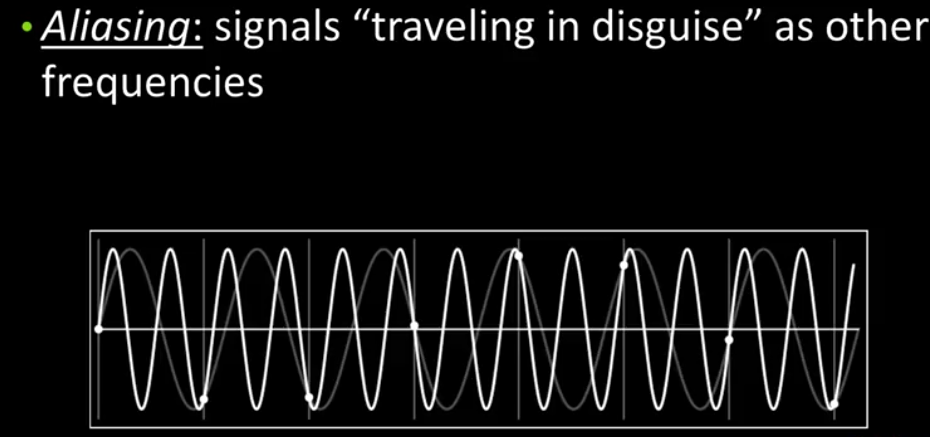
By the way, this also happens in time. Have you ever watched a video where an airplane propeller is starting to go? And then all of a sudden st, you start to kind of see it's spinning backwards, and then you see it spinning forwards.

Okay, airplane propellers don't spin backwards. They only go forwards. So what's going on there? Oh, and by the way, I hope you know that if you were actually standing out on the tarmac, watching the airplane, you wouldn't see this phenomenon. The reason you're seeing this phenomena is that this was recorded on either video or film that was taking a picture every so often, and that's what's displayed here. Imagine we have this wheel that's turning this amount each time. So if you track the dot, you can see that the thing is turning almost 90 degrees at every rotation. But, if that dot wasn't there, you would actually see this thing going backwards just a little bit. Because of the fact that you couldn't tell which one of those cross patterns was which, and so you would see it rotating backwards, okay? And that's aliasing in the temporal domain. We'll, we'll talk about that in a minute in the spatial domain. And essentially, the thing is moving too fast for how often you're sampling a time for you to actually be able to tell what's going on. The high frequency and the low frequency can't be distinguished.

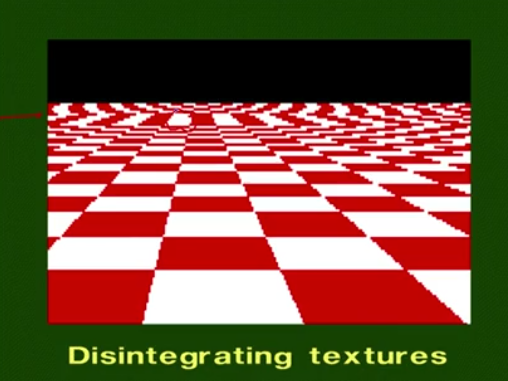
To show you a simple example in an artificial image, we'll see some natural ones later. Here we have a rendering, and as this checkerboard gets further away from you in the distance, right? It's supposed to start getting thinner and thinner and closer and closer. And you'll notice, that somewhere right around here, it starts to break up. It's not looking like a checkerboard look. In fact, look at this nonsense, right? It's like low frequency all over again. What's going on?

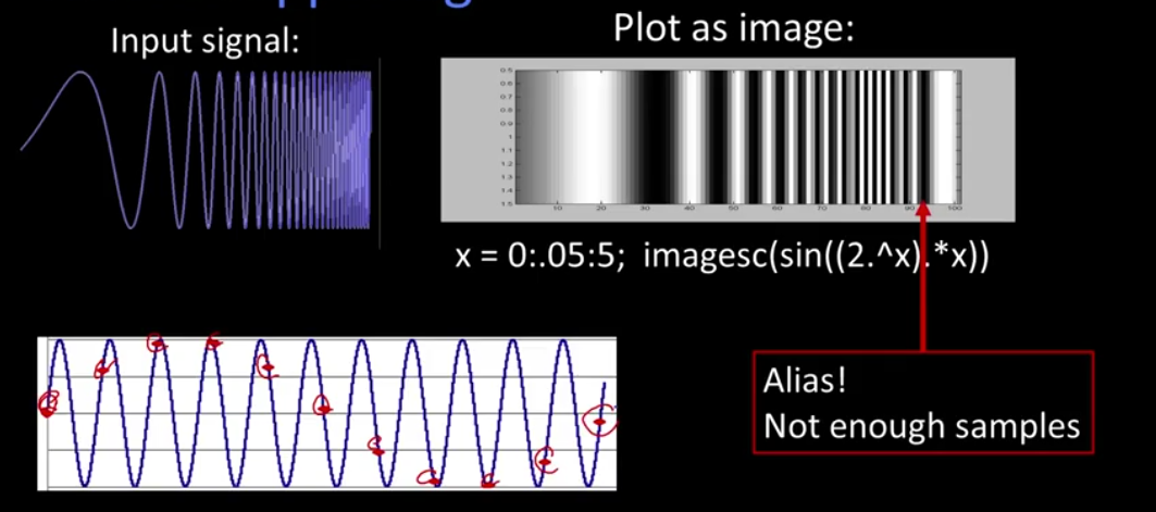
Well, we can look at that in MATLAB, all right? Suppose we have this input signal. Okay, this is like that chirp that I was showing you before. Well, we can plot this as an image in MATLAB, and that would look like this, okay? So here I'm just doing the x from zero to five by 0.05, and I'm, I did this image of sine of 2 to the x times x, all right? And, what you're seeing is, so it starts off a slow frequency, and then it's getting higher and higher and, eventually, you start to see stuff that looks like that. So what's going on there? Well, that's aliasing. There are not enough pixels in the, in the plot for you to be able to see what's going on. And that's illustrated down here, where we have a small number of samples, a not dense enough sampling, in order to recover those frequencies.