Understanding Diagonals, Off-Diagonals, and Loss Functions in Siamese Networks

Introduction

In our previous discussion on Siamese networks, we briefly mentioned diagonals and off-diagonals in the cost matrix. Now, let’s dig deeper to understand what they mean, how they relate to duplicate detection, and how they influence your loss function during training.

What Are Diagonals and Off-Diagonals?

When we train a Siamese network, we usually divide the training data into two batches — each containing unique, non-duplicate questions. These batches are passed through twin subnetworks that output embedding vectors for each question.

For example, suppose each question is represented by a vector of dimension 1 x d_model. The similarity between every pair of embeddings (from the two batches) forms a similarity matrix.

• Diagonal values (green) → Similarities of duplicate questions

• Off-diagonal values (orange) → Similarities of non-duplicate questions

Ideally, the diagonal values should be higher because duplicates should produce more similar embeddings.

In the last blog, I briefly mentioned the diagonals and the off diagonals in our cost matrix. We will now define these terms and use them to compute the overall costs. Let's dive in. Previously you set up the training data into two specific batches. Each batch containing no duplicate questions within it. You ran those batches through one subnetwork each, and that's produced a vector outputs per question, which has dimension one by d model. Where d model is the embedding dimension and is equal to the number of columns in the matrix, which is five, at least in this example, the v_1 vectors for a single batch are stack together. In this case, the batch size is the number of rows shown in this matrix, which is four. You can see a similar batch of v_2 vectors as well. The last step was to combine the two branches of the Siamese network by calculating the similarity between all vector pair combinations of the v_1 vectors and v_2 vectors.

For this example with a batch size of four, that last step would produce a matrix of similarities that looks something like this. This matrix has some important attributes. The similarities along the green diagonal contains similarities for the duplicate questions. For a well-trained model, these values should be greater than similarities for the off-diagonals, reflecting the fact that the network produces similar vector outputs for duplicate questions. The orange values in the upper-right and lower-left are similarities for the non-duplicates questions. Now, this is where things get really interesting. You can use this off-diagonal information to make some modifications to the loss function and really improve your model's performance.

Mean Negative: Averaging Off-Diagonals

The mean negative is the average of all off-diagonal values in a row.

Even though some of these off-diagonal values can be positive, they represent negative examples. Taking their mean helps us reduce noise during training.

By replacing the individual negative similarities with the mean negative in the loss function, we make the model converge faster and train more stably.

To do so, I'm going to make use of two concepts. The first concept is the mean negative, which is just the mean or average of all the off-diagonal values in each row. Notice that off-diagonal elements can still be positive numbers. When I say mean negative, I'm referring to the mean of the similarity for negative examples, not the mean of negative numbers in a row. For example, the mean negative of the first row is just the mean of all the off-diagonal values in that row. In this case, negative 0.8, 0.3, and negative 0.5, excluding the value 0.9, which is on the diagonal. You can use the mean negative to help speed up training by modifying the loss function, which I'll show you soon.

Closest Negative: Finding the Hard Example

The closest negative is the off-diagonal value closest to (but still less than) the diagonal value for that row.

This represents the hardest negative example — the one that is most similar to the positive example. Focusing on these hard negatives forces the network to better learn the difference between duplicates and non-duplicates.

The next concept is what's called the closest negative. As mentioned earlier, because of the way you define the triplet loss function, you'll need to choose so-called hard triplets to train on. What this means is that for training, you want to choose triplets where the cosine similarity of the negative example is close to the similarity of the positive example. This forces your model to learn what differentiates these examples and ultimately drive those similarity values further apart through training. To do this, you will search each row in your outputs matrix for the closest negative, which is to say, the off-diagonal value which is closest to, but still less than the value on the on-diagonal for that row. In this first row, the value on the diagonal is 0.9. The closest off-diagonal elements, in this case, is 0.3. What this means is that this negative example with a similarity of 0.3 has the most to offer your model in terms of learning opportunity. To make use of these new concepts, recall that the triplet loss was defined as the max of the similarity of A and N minus the similarity of A and P plus the margin Alpha and zero. Also, recall that we referred to the difference between the two similarities with the variable named diff.

Updating the Triplet Loss

Here, we're just writing out the definition of diff. In order to minimize the loss, you want this diff plus the margin Alpha to be less than or equal to zero. I'll introduce loss one to be the max of the mean negative minus the similarity of A and P plus Alpha and zero. The change between the formulas for triplet loss and loss one is the replacement of similarity of A and N. With the mean negative, this helps the model converge faster during training by reducing noise. It reduces noise by training on just the average of several observations rather than training the model on each of these off-diagonal examples. Why does taking the average of several observations usually reduce noise? Well, we define noise to be a small value that comes from a distribution that is centered around zero. In other words, the average of several noise values is usually zero. If we took the average of several examples, this has the effect of canceling out the individual noise from those observations. Then, last two will be the max of the closest negative minus the similarity of A and P plus Alpha and zero. The difference between the formulas, this time, is the replacement of the cosine of A and N with the closest negative, this helps create a slightly larger penalty by diminishing the effects of the otherwise more negative similarity of A and N that it replaces. You can think of the closest negative as finding the negative example that results in the smallest difference between the two cosine similarities. If you had that small difference to Alpha, then you are able to generate the largest loss among all of the other examples in that row.

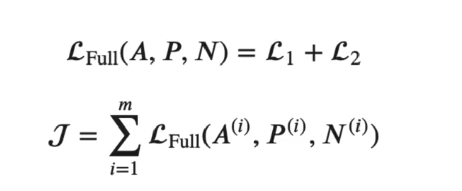
By focusing the training on the examples that produce higher loss values, you make the model update its weights more. To learn from these more difficult examples, then you can define the full loss as loss 1 plus loss 2. You will use this new full loss as an improved triplet loss in the assignments. The overall costs for your Siamese network will be the sum of these individual losses over the training sets. In the next video, you will use this cost function in one-shot learning. One-shot learning is a very effective technique that can save you a lot of time when comparing the authenticity of checks or of any other type of inputs.

Why This Matters

By using both the mean and closest negative, your Siamese network:

• Learns faster by reducing training noise

• Focuses on challenging examples

• Produces more accurate embeddings for similarity-based tasks

This approach is especially useful in one-shot learning, where you need to quickly identify whether two inputs (like handwritten digits, faces, or text questions) are similar or not.