🧠 5 Powerful Model Selection and Preprocessing Techniques in Scikit-Learn (With Simple Python Examples)

Working with machine learning in Python often means making smart choices — not just about models, but about how you prepare data, interpret results, and fine-tune predictions.

In this post, we’ll walk through five essential techniques in scikit-learn that go beyond basic model fitting. These are:

• Model Calibration

• Permutation Importance

• FeatureHasher

• RobustScaler

• FeatureUnion

We’ll keep things simple and include clear Python code using built-in datasets, so you can try them out right away.

1. ✅ Model Calibration: Making Probabilities Reliable

When we develop a machine learning classifier model, we need to remember that it’s not enough simply to provide correct classification prediction; the probabilities associated with the prediction must also be reliable. The process to ensure that the probabilities are reliable is called calibration.

The calibration process adjusts the model’s probability estimation. The technique pushes the probability to reflect the true likelihood of the prediction so it is not overconfident or underconfident. The uncalibrated model might predict an event with a 90% probability chance, while the actual success rate is much lower, which means the model was overconfident. That’s why we need to calibrate the model.

Sometimes classifiers (like RandomForest or SVM) give probability scores that aren’t well-calibrated. That means the model says there’s an 80% chance of something happening — but it only happens 60% of the time.

Model calibration helps fix that. It aligns predicted probabilities with actual outcomes.

🔍 Use Case

Useful when probability confidence matters — like in medical diagnosis or fraud detection.

from sklearn.inspection import permutation_importance
result = permutation_importance(model, X_test, y_test, n_repeats=10, random_state=42)
# Display top 5 important features
import numpy as np
indices = np.argsort(result.importances_mean)[-5:]
for i in indices[::-1]:
 print(f"Feature {i}: Importance = {result.importances_mean[i]:.4f}")

🔎 Try combining this with SHAP or LIME for deeper interpretation.

import numpy as np
import matplotlib.pyplot as plt
from sklearn.datasets import load_breast_cancer
from sklearn.linear_model import LogisticRegression
from sklearn.calibration import calibration_curve, CalibratedClassifierCV
from sklearn.model_selection import train_test_split
data = load_breast_cancer()
X, y = data.data, data.target
X_train, X_test, y_train, y_test = train_test_split(X, y, random_state=42)
lr = LogisticRegression().fit(X_train, y_train)
prob_pos_lr = lr.predict_proba(X_test)[:, 1]
fraction_lr, mean_pred_lr = calibration_curve(y_test, prob_pos_lr, n_bins=10)
calibrated_clf = CalibratedClassifierCV(lr, cv='prefit', method='isotonic')
calibrated_clf.fit(X_train, y_train)
prob_pos_calibrated = calibrated_clf.predict_proba(X_test)[:, 1]
fraction_cal, mean_pred_cal = calibration_curve(y_test, prob_pos_calibrated, n_bins=10)
plt.figure(figsize=(8, 6))
plt.plot(mean_pred_lr, fraction_lr, marker='o', label='Original LR')
plt.plot(mean_pred_cal, fraction_cal, marker='s', label='Calibrated LR (Isotonic)')
plt.plot([0, 1], [0, 1], linestyle='--', label='Perfect Calibration')
plt.xlabel("Mean predicted probability")
plt.ylabel("Fraction of positives")
plt.title("Calibration Curve Comparison")
plt.legend(loc="upper left")
plt.show()

We can see that the calibrated logistic regression is closer to the model with perfect calibration than the original. This means that the calibrated model can better estimate the actual risk, although it is still not ideal.

Try using the calibration method to improve the model prediction capability.

2. 🧪 Permutation Importance: Know What Really Matters

Whenever we work with a machine learning model, we use the data features to provide the prediction result. However, not every feature contributes to the prediction in the same manner.

he permutation_importance() method is for measuring the feature contribution to model performances by randomly permuting (changing) feature values and evaluating the model performance after the permutation. If the model performance degrades, the feature impacts the model; conversely, if the model performance is unchanged, it suggests that the feature might not be that useful for the specific model performance.

The technique is straightforward and intuitive, making it helpful in interpreting any model’s internal decision-making. It’s beneficial for models with no inherent feature importance method embedded inside.

Feature importance from models like RandomFores. t is often biased. Permutation importance gives a model-agnostic way to evaluate how each feature impacts performance — by randomly shuffling feature values and seeing how the score changes.

🧪 Python Example 1

from sklearn.inspection import permutation_importance
result = permutation_importance(model, X_test, y_test, n_repeats=10, random_state=42)
# Display top 5 important features
import numpy as np
indices = np.argsort(result.importances_mean)[-5:]
for i in indices[::-1]:
 print(f"Feature {i}: Importance = {result.importances_mean[i]:.4f}")

🧪 Python Example 2

import numpy as np
import matplotlib.pyplot as plt
from sklearn.datasets import load_iris
from sklearn.linear_model import LogisticRegression
from sklearn.inspection import permutation_importance
from sklearn.model_selection import train_test_split
data = load_iris()
X, y = data.data, data.target
X_train, X_test, y_train, y_test = train_test_split(X, y, random_state=42)
model = LogisticRegression()
model.fit(X_train, y_train)
result = permutation_importance(model, X_test, y_test, n_repeats=10, random_state=42, scoring='accuracy')

With the code above, we have the model and permutation importance result, where we will analyze the feature’s impact on the model. Let’s look at the average and standard deviation results for permutation importance.

feature_names = data.feature_names
importances = result.importances_mean
std = result.importances_std
for i, name in enumerate(feature_names):
 print(f"{name}: Mean importance = {importances[i]:.4f} (+/- {std[i]:.4f})")

plt.barh(feature_names, importances, xerr=std)
plt.xlabel("Decrease in accuracy")
plt.title("Permutation Importance")
plt.show()

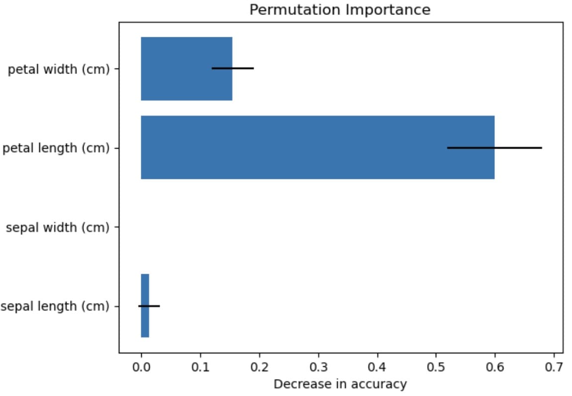
The visualization shows that the petal length most impacts the feature performance, while the sepal width has no effect. There is always uncertainty, which is represented by the standard deviation, but we can conclude with the permutation importance technique that petal length has the most impact.

That’s a simple feature importance technique that you can use for your next project.

3. 🔢 FeatureHasher: Handle High-Cardinality Categorical Data

Working on features for data science modeling, I often found that high-dimensional features were too memory intensive, which impacted the application’s overall performance. There are many ways to improve performance, such as dimensionality reduction or feature selection. The hashing method is another method that might be rarely used but could be helpful.

Hashing is converting data into a sparse numeric matrix with a fixed size. Applying a hash function to each feature can map the represented feature into a sparse matrix. We will use a hash function via FeatureHasher to compute the matrix column corresponding to a name.

When you have text categories with thousands of unique values (like ZIP codes or URLs), one-hot encoding becomes impractical. FeatureHasher provides a memory-efficient alternative.

from sklearn.feature_extraction import FeatureHasher
data = {'feature': 'dog'}, {'feature': 'cat'}, {'feature': 'rabbit'}
hasher = FeatureHasher(n_features=5, input_type='string')
hashed_features = hasher.transform([d.values() for d in data])
print(hashed_features.toarray())

import pandas as pd
import seaborn as sns
from sklearn.feature_extraction import FeatureHasher
titanic = sns.load_dataset("titanic")
titanic_sample = titanic[['sex', 'embarked', 'class']].dropna()
data_dicts = titanic_sample.to_dict(orient='records')
hasher = FeatureHasher(n_features=10, input_type='dict')
hashed_features = hasher.transform(data_dicts)
hashed_array = hashed_features.toarray()
print("\nHashed feature matrix (dense format):\n", hashed_array)

4- 🔄 RobustScaler: Handle Outliers Gracefully

Real-world data is rarely clean, and more often than not riddled with outliers. While an outlier is not intrinsically bad and might give information that contributes to the actual insight, there are times when it will skew our model results.There are many techniques for scaling our outliers, but sometimes they can introduce bias. That’s why robust scaling is important to help preprocess our data. Robust scaling transforms the data by removing the median and scaling them according to the IQR instead of using mean and standard deviation.The robust scaler is proper, with only a few outliers at extreme positions. By applying it, the dataset is stable and not influenced much by the outliers, which makes it useful for any machine learning model development. Here is an example of using the robust scaler. Let’s use the Iris data example and introduce an outlier in the dataset.

import numpy as np
import pandas as pd
from sklearn.datasets import load_iris
from sklearn.preprocessing import robust_scale
import matplotlib.pyplot as plt
iris = load_iris()
X = iris.data
outlier = np.array([[10, 10, 10, 10]])
X_out = np.vstack([X, outlier])
X_scaled = robust_scale(X_out)

from sklearn.preprocessing import RobustScaler
import numpy as np
X = np.array([[10], [100], [1000], [10000]])
scaler = RobustScaler()
X_scaled = scaler.fit_transform(X)
print(X_scaled)

5. 🧩 FeatureUnion: Combine Multiple Transformers

If you want to apply different preprocessing steps in parallel and merge their outputs, use FeatureUnion. It’s like Pipeline, but for combining, not chaining. Feature union is a Scikit-Learn feature that combines multiple feature transformations within the pipeline. Instead of transforming the same features sequentially, feature union inputs the data into several transformers simultaneously to provide all the transformed features. It’s a helpful feature where different transformers are required to capture various aspects of data and need to be present in the dataset. One transformer might used for the PCA technique, while the others use robust scaling.Let’s try it out with the following code below. For example, we can create transformers for both PCA and polynomial features transformers.

from sklearn.pipeline import FeatureUnion
from sklearn.preprocessing import StandardScaler, PolynomialFeatures
union = FeatureUnion([
 ('std', StandardScaler()),
 ('poly', PolynomialFeatures(degree=2, include_bias=False))
])
X = np.array([[1, 2], [3, 4], [5, 6]])
X_transformed = union.fit_transform(X)
print(X_transformed)

References

1-6 Lesser-Known Scikit-Learn Features That Will Save You Time