Understanding Vanilla RNNs: How They Work and Propagate Information Over Time

 

Title Tag:
How Vanilla RNNs Work | Forward Propagation Explained Simply

Meta Description:
Learn how vanilla RNNs process sequences and make predictions over time. Includes a breakdown of forward propagation and the role of hidden states in RNNs

you saw the advantages and the basic idea behind your current neural networks. RNNs might seem like complicated structures, but as you will see, their computations are actually pretty straight forward. I'll show you how plain RNNs propagates information through time within a sequence of variables, as well as how they make sequential predictions.

Recurrent Neural Networks (RNNs) might look a bit complex at first, especially compared to feedforward networks. But once you break them down, their computations are surprisingly straightforward.

In this post, we’ll walk through:

• The basic structure of a vanilla RNN

• How it processes sequences over time

• The forward propagation steps and the underlying math

Sections

• What Is a Vanilla RNN?
• RNN Architecture: A Quick Overview
• Forward Propagation Equations
• Step-by-Step: How RNNs Compute Predictions
• The Role of Hidden States
• What It Does:

What Is a Vanilla RNN?

At its core, a vanilla RNN (also called a plain or simple RNN) is a neural network designed to handle sequential data. Think of sequences like:

• Words in a sentence

• Time-series data

• Audio waveforms

The idea is that RNNs remember what happened before (via hidden states) and use that information to influence predictions later in the sequence.

You'll get familiar with the math behind basic recurrent units, to prepare you to implement forward propagation in RNN. Take a look at this plain or vanilla RNN, it has too many architecture.

RNN Architecture: A Quick Overview

Here’s how the architecture works:

At each time step t, the RNN takes:

• An input vector $x^{(t)}$ (e.g., the current word)

• A hidden state $h^{(t-1)}$ from the previous time step

Then it calculates:

1. A new hidden state $h^{(t)}$

2. A prediction $\hat{y}^{(t)}$

So at each side step it takes an X, a hidden states H and makes a prediction Y hat. Additionally, it propagates in new hidden state to the next time step.

Forward Propagation Equations

1. Hidden state update:

   $$h^{(t)} = \tanh(W_{hx} \cdot x^{(t)} + W_{hh} \cdot h^{(t-1)} + b_h)$$

2. Prediction:

   $${\widehat{y}}^{(t)}=\text{softmax}(W_{yh}\cdot h^{(t)}+b_y)$$

The hidden state helps carry memory forward, so the model can learn from what came earlier in the sequence.

The hidden states at every time T, is computed with an activation function G, with arguments equal to the products between a premature matrix W, subscript H and the previous hidden states H, superscript T minus 1. These are concatenated with the input variable X superscript T, plus the bias term. The complete equation looks like this, where X superscript T and H superscript T minus 1, are multiplied by different parameters, and the resulting vectors are summed up element twice.

After computing the hidden state at time T, it's possible to get the prediction Y hat by using an activation function G, with arguments equal to the product between the head and state, and some parameters W plus a bias trim. These two equations together represent all of the math behind a simple arnon,

Step-by-Step: How RNNs Compute Predictions

Let’s walk through the flow inside a single RNN cell (or time step):

1. Inputs:

   • The input at time $t$, $x^{(t)}$

   • The previous hidden state $h^{(t-1)}$

2. Compute the new hidden state:

   • Multiply $x^{(t)}$ with its weight matrix.

   • Multiply $h^{(t-1)}$ with a different weight matrix.

   • Add both results and a bias term.

   • Apply a non-linear activation function like tanh.

3. Make a prediction:

   • Multiply the new hidden state with output weights.

   • Add a bias.

   • Apply softmax (or another suitable activation).

This process repeats for each element in the sequence, passing the hidden state forward each time.

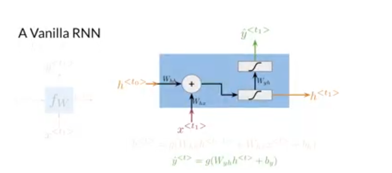
but let's take a detailed look at the order in which competitions are made. Let's focus on the first cell from the RNN. It takes as input the previous hidden state and the current variable X, which might be the first word in a sentence. To get the current hidden states first, you have to get the products of X and H, superscript T sub 0 with the respective parameters, and then sum the vector's element twice. Next, pass the resulting vector through an excavation function, with the resulting value you can compute the current Y hat. Now by multiplying the current hidden state, with a set of learnable parameters W subscript YH, and going through another excavation function. In the literature related to RNN you'll find similar diagrams to what you see here, which show the order of computation, and how information is propagated within a recurrent unit.

The Role of Hidden States

The hidden state is the heart of an RNN. It allows the network to remember previous inputs and use that context for the current prediction.

In NLP, this is crucial for understanding language. For example, knowing the previous words in a sentence helps the model predict the next one more accurately.

It is important for you to take away that hidden states are the variables that allow RNNs to propagate information through time, or in other words through different positions within the sequence. As you saw at every step, recurrent units have two inputs. You now know the feet forward equations and the cost function for an RNN. In the next video, I'll show you how the cost function for the RNN works

What It Does:

• Simulates a sequence of 3 steps.

• Computes new hidden states and predictions at each step.

• Shows how information flows through time.

References