[MUSIC] In this module, we've discussed how to think about two dimensional functions as landscapes. And we've also seen that we can construct Jacobian vectors which tell us both the direction and the magnitude of the gradient at each point in space. Last video, we added one further tool to our toolbox, which allowed us to double check what kind of feature we were standing on, when we landed on a point with a 0 gradient. These concepts will all be very useful to develop your understanding of optimisation problems, and have also let you see why multivariate calculus is worth knowing. However, in this video we are going to remind ourselves about two features of real systems which so far, we've avoided. Firstly for many applications of optimisation such as in the training in neural networks, you are going to be dealing with a lot more than two dimensions potentially hundreds or thousands of dimensions. This means that we can no longer draw a nice surface and climb its mountains. All the same maths still applies but we now have to use our 2D intuition to guide and enable us to trust the maths. Secondly, as we've mentioned briefly before, even if you do just have a 2D problem, very often you might not have a nice analytical function to describe it and calculating each point could be very expensive. So even though in principle a plot could possibly be drawn, you wouldn't be able to afford either the super computer time or perhaps the laboratory staff to fully populate this thing. Thirdly, all the lovely functions that we've dealt with so far were smooth and well-behaved. However, what if our function contains a sharp feature like a discontinuity? This would certainly make navigating the sand pit a bit more confusing. Lastly, there are a variety of factors that may result in a function being noisy. Which, as I'm sure you can you imagine, might make our Jacobian vectors pretty useless unless we were careful. So this brings us nicely to the second topic in this video, which is a question that I hope you've all been screaming at your screens for the past few minutes. If, as I said a minute ago, we don't even have the function that we're trying to optimise, how on earth are we supposed to build a Jacobian out of the partial derivatives? This is an excellent question, and leads us to another massive area of research called numerical methods. There are many problems, which either don't have a nice explicit formula for the answer, or do have a formula but solving it directly would take until the end of time. To fight back against the universe mocking us in this way, we have developed a range of techniques that allow us to generate approximate solutions. One particular approach, and it's relevant to our discussion of the Jacobian actually takes us right back to the first few lectures on this course where we defined the derivative.

We started by using an approximation based on the rise over run, calculated over a finite interval. And then looked at what happened as this interval approached 0. All we're doing with the finite difference method is accepting that we're not going to work out the value of the function at every single point in space. So we're just going to use the points that we do have and build an approximation for the gradient based on that.

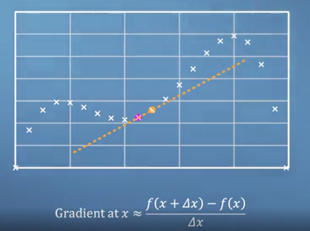
In the example shown here, we have already calculated lots of points on this one dimensional function, but clearly that's not going to be practical for high-dimensional scenarios. So all we do is take this logic one step further and say, if we start from an initial location, and we would like to approximate the Jacobian, we will simply approximate each partial derivative in turn. So taking a small step in x allows us to calculate an approximate partial derivative in x. And a small step in y gives an approximate partial in y. Two things to bear in mind here. Firstly, how big should our little step be? Well, this has to be a balance. because if it's to big you'll make a bad approximation for reasons that I hope will be obvious by this point. But if it's too small, then we might run into some numerical issues. Just remember, when your computer calculates the value of the function at a point, it only stores it to a certain number of significant figures. So if your point is too close, your computer might not register any change at all. Second, as we mentioned earlier, what happens if your data is a bit noisy? To deal with this case, many different approaches have been developed.

But perhaps the simplest is just to calculate the gradient using a few different step sizes and take some kind of average. This brings us to the end of this video. So I hope you can see that once we leave the world of nice smooth functions, and into the real world of noisy data and computationally expensive functions, things start to get a lot more interesting. See you next time. [MUSIC]