

Steps involved in Building a Machine Learning Model




Test
The goal of machine learning is to discover patterns and relationships in data and put those findings to use. This process of discovery is achieved through the use of modeling techniques that have been developed over the past 30 years in statistics, computer science and applied mathematics [1]. These different approaches can range from simple to extremely complex, but they all share a common goal: to estimate the functional relationship between the input characteristics and the target variable. Building a successful machine-learning model involves the following steps:
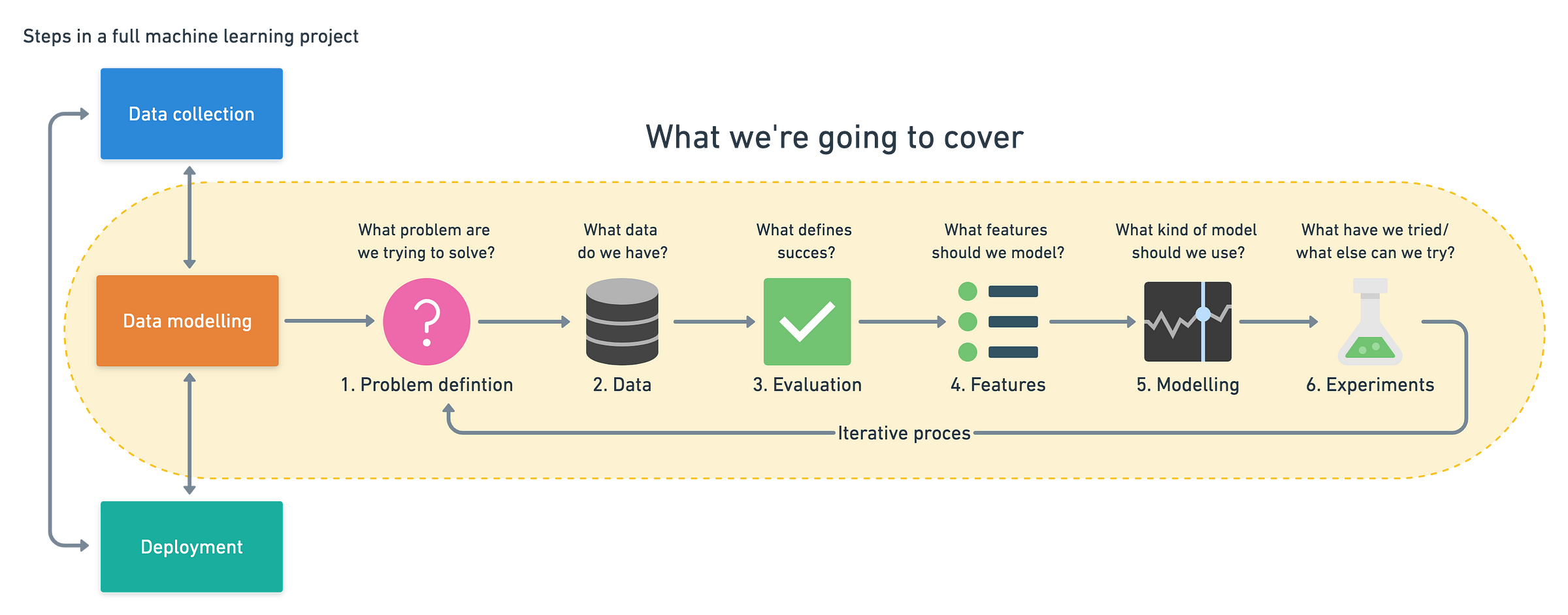

- Data Preparation
- Model Selection
- Model Training
- Validation
- Hyperparameter Tuning
1- Data Preparation or Preprocessing
A crucial component of machine learning is the availability of large and labeled datasets. These datasets serve as the training data for ML algorithms, allowing them to learn patterns and make accurate predictions. Datasets can vary based on the problem domain, such as images, text, audio, or a combination of different data types.
Data is a crucial component of deep learning. A dataset refers to a collection of examples or instances used to train, validate, and test deep learning models. Datasets can include images, text, audio, video, or any other type of information relevant to the task at hand.
The first step in building a machine learning model is to gather and prepare the data. This includes cleaning, transforming, and scaling the data. In data science, data cleaning is the process of identifying incorrect data and fixing the errors so the final dataset is ready to be used. Errors could include duplicate fields, incorrect formatting, incomplete fields, irrelevant or inaccurate data, and corrupted data.

1. 1- Historical data or Rawa Data
As shown in the image above, the machine learning process usually begins with collecting historical data. Then, this data is prepared to fit into a machine-learning model[1]
1.2- Creating New Features
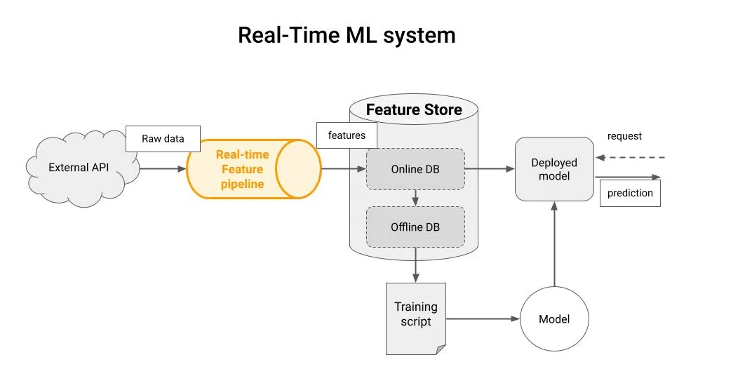
Creating new features is an important step in feature engineering that involves creating new variables or columns from existing data. This can help to capture complex relationships between the features and improve the accuracy of the models. Here are some techniques for creating new features[2]:
1. Interaction features: Interaction features are created by multiplying two or more existing features together. This can help to capture the joint effects of the features and uncover new patterns in the data. For example, if we have two features, “age” and “income”, we can create a new interaction feature called “age_income” by multiplying these two features together.
2. Polynomial features: Polynomial features are created by raising existing features to a higher power. This can help to capture non-linear relationships between the features and improve the accuracy of the models. For example, if we have a feature “age”, we can create a new polynomial feature called “age_squared” by squaring this feature.
3. Binning: Binning involves grouping continuous values into discrete categories. This can help to capture non-linear relationships and reduce the impact of outliers in the data. For example, if we have a feature “age”, we can create a new binned feature called “age_group” by grouping the ages into different categories such as “0–18”, “18–25”, “25–35”, “35–50”, and “50+”.
1.3- Encoding Categorical Variables
Encoding categorical variables is a crucial step in feature engineering that involves converting categorical variables into a numerical form that machine learning algorithms can understand. Here are some common techniques used for encoding categorical variables:[2].
One-Hot Encoding:
One-hot encoding is a technique that converts categorical variables into a set of binary features, where each feature corresponds to a unique category in the original variable. In this technique, a new binary column is created for each category, and the value is set to 1 if the category is present and 0 if not [2].
Label Encoding:
Label encoding is a technique that assigns a unique numerical value to each category in the original variable. In this technique, each category is assigned a numerical label, where the labels are assigned based on the order of the categories in the variable[2].
Ordinal Encoding
Ordinal encoding is a technique that assigns a numerical value to each category in the original variable based on their order or rank. In this technique, the categories are ordered based on a specific criterion, and the categories are assigned numerical values based on their position in the order[2].
1.4- Handling Imbalanced Data
Dealing with imbalanced data is an important aspect of machine learning. Imbalanced data is a situation where the distribution of the target variable is not uniform, and one class is underrepresented compared to the other. This can lead to a bias in the model toward the majority class, and the model may perform poorly on the minority class. Some of the techniques to handle imbalanced data are[2].
1. Upsampling: Upsampling involves creating more samples for the minority class by resampling the existing samples with replacement. This can be done using the resample function from the sklearn.utils module.
2. Downsampling: Downsampling involves removing some samples from the majority class to balance the distribution. This can be done using the resample function from the sklearn.utils module.
3. Synthetic Minority Over-sampling Technique (SMOTE): SMOTE involves creating synthetic samples for the minority class based on the existing samples. This can be done using the SMOTE function from the imblearn.over_sampling module.
4. Class Weighting: Class weighting involves assigning a weight to each class in the model to account for the imbalance. This can be done using the class_weight the parameter in the model.
5. Anomaly Detection: Anomaly detection involves identifying the outliers in the data and removing them. This can be done using the IsolationForest function from the sklearn.ensemble module. Anomaly detection identifies rare events or observations in a dataset that deviate significantly from the expected or normal behavior. In the case of imbalanced data, where the number of observations in one class is much lower than the other, anomaly detection can be used to identify and label the rare observations in the minority class as anomalies. This can help balance the dataset and improve the performance of machine learning models.
6. Cost-Sensitive Learning: Cost-sensitive learning involves assigning a different cost to each type of error in the model to account for the imbalance. This can be done using the sample_weight the parameter in the model.
1.5- Skewness and Kurtosis Handling
Skewness and kurtosis are statistical measures that can help in understanding the distribution of data. Skewness measures the degree of asymmetry in the data, while kurtosis measures the degree of peakedness or flatness of the distribution[2]
Skewed data can negatively affect the performance of machine learning models. Therefore, it is important to handle skewness in the data. Here are some techniques to handle skewness in the data:
- Log transformation: Logarithmic transformation can be used to reduce the skewness of data. It can be applied to both positively and negatively skewed data.
- Square root transformation: The square root transformation can be used to reduce the skewness of data. It can be applied to positively skewed data.
- Box-Cox transformation: The Box-Cox transformation is a more general transformation method that can handle both positively and negatively skewed data. It uses a parameter lambda to determine the type of transformation to be applied to the data.
Handling kurtosis can be done by applying a transformation similar to that used for handling skewness. Some techniques for handling kurtosis include:
- Log transformation: Logarithmic transformation can also be used to handle kurtosis in the data.
- Square transformation: The square transformation can also be used to handle kurtosis in the data.
- Box-Cox transformation: The Box-Cox transformation can also be used to handle kurtosis in the data.
1.6- Handling Rare Categories
Handling rare categories refers to the process of dealing with categories in categorical variables that occur infrequently in the data. Rare categories can cause problems in machine learning models, as they may not have enough representation in the data to be accurately modeled. Some techniques for handling rare categories are [2]:
- Grouping the rare categories: This involves grouping rare categories into a single category or a few categories. This reduces the number of categories in the variable and increases the representation of the rare categories.
- Replacing the rare categories with a more common category: This involves replacing the rare categories with the most common category in the variable. This can be effective if the rare categories are not important for the analysis.
- One-hot encoding with a flag: This involves creating a new category for rare categories and flagging them as rare. This allows the model to treat rare categories differently from other categories.
1.7-Scaling and Normalization
Scaling and Normalization are important steps in feature engineering to ensure that the features are on a similar scale and have similar ranges. This can help improve the performance of some machine learning algorithms and make the optimization process faster. Here are some common techniques used for scaling and normalization [2]
1. Standardization: Standardization scales the features so that they have zero mean and unit variance. This is done by subtracting the mean from each value and then dividing it by the standard deviation. The resulting values will have a mean of zero and a standard deviation of one.
2. Min-Max Scaling: Min-Max scaling scales the features to a fixed range, usually between 0 and 1. This is done by subtracting the minimum value from each value and then dividing by the range.
3. Robust Scaling: Robust scaling is similar to standardization, but it uses the median and interquartile range instead of the mean and standard deviation. This makes it more robust to outliers in the data.
4. Normalization: Normalization scales each observation to have a unit norm, which means that the sum of squares of each feature value is 1. This is useful for some algorithms that require a similar scale for all samples.
1.8 Data Splitting
Generally, a dataset should be split into Training and Test sets with a ratio of 80 percent Training set and 20 percent test set. This split of the Training and Test sets is ideal.

What is Training Data?
All the machine learning algorithms learn from data by finding relationships, developing understanding, making decisions, and building its confidence by using the training data we provide to a machine learning model. And this is to be noted that a machine learning model will perform based on what training data we have given to a model. The more training data we will provide, the better the model will perform.
What is Test Data?
Once a machine learning model is trained by using a training set, then the model is evaluated on a test set. The test data provides a brilliant opportunity for us to evaluate the model. The test set is only used once our machine learning model is trained correctly using the training set. Generally, a test set is only taken from the same dataset from where the training set has been received.
Validation Set
Besides the Training and Test sets, there is another set which is known as a Validation Set. A validation Set is used to evaluate the model’s hyperparameters. Our machine learning model will go through this data, but it will never learn anything from the validation set. A Data Scientist use the results of a Validation set to update higher level hyperparameters.
I will just say that some models need substantial data to be trained with, in some cases models with very few hyperparameters will be easy to validate and prepare, in such instances, you need to split the data into three sets. Still, the ratio of the validation set should be less if you have few
If your model has many hyperparameters, then obviously you need to increase the proportion of validation set. In some cases, when your model will not have any hyperparameters, in such cases, you will not need a Validation Set.
2- Model Selection
After data preparation, the next step is to choose an appropriate machine-learning algorithm for the task. The choice of algorithm will depend on the type of problem being solved.
A typical question asked by a beginner, when facing a wide variety of machine learning algorithms, is “which algorithm should I use?” The answer to the question varies depending on many factors, including:
- The size, quality, and nature of data.
- The available computational time.
- The urgency of the task.
- What you want to do with the data.
3- Model Training
Once an algorithm has been selected, it needs to be trained using a subset of the data.
4- Validation
Validation involves testing the trained model on a separate dataset to evaluate its performance.
5-Hyperparameter Tuning
Hyperparameters are settings that govern how the machine learning algorithm works. Tuning these hyperparameters can improve model performance.
References
2-The Ultimate Guide to Machine Learning: Feature Engineering — Part -2